Introduction:

Sooner of later in your hobby or career in electronic circuit design, you will encounter feedback. The concepts of feedback is critical to your ability to design good circuits and systems. It is a shame that many practicing engineers (and even some professors) have little appreciation of the foundations of feedback. In whatever little professional experience I had as a circuit designer, never a day passed without encountering feedback in some form or the other. Here we will briefly discuss feedback in single input, single output, time-invariant, linear continuous-time systems (a fancy term to which most of your circuits would neatly approximate.

What happened in the past:

Armstrong's Regenerative Amplifier

Given that you see positive feedback so little in circuits today (except oscillators, may be), you will be surprised to learn that the first electronic applications of feedback at the beginning of 20th century were all of the positive kind. Robert Goddard used positive feedback in his vacuum tube oscillators and Edwin Armstrong used it to increase the voltage gain in his amplifiers (also made from vacuum tubes). Armstrong's amplifier (called the regenerative amplifier) was remarkable in obtaining large gains from a single stage amplifier which others could only do by a cascade of multiple amplifiers. Thus his design was cheaper. Lets understand a block diagram of how he achieved this.

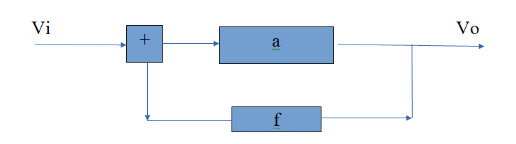
I leave it as an exercise to my smart readers to do some algebra and derive that Vo = a/(1-af) * Vi

So the so called closed loop gain A = Vo/Vi = a/(1-af)

Here,

a is the open loop gain of a single amplifier

f is the fraction of the output voltage fed back to the amplifier input. It is implemented by passive elements.

Clearly, for af < 1, the overall closed loop gain A will be greater than a. For, af = 0.9, we get an increase of 10 times, for af = 0.09, we get an increase of 100 times. Thus, Armstrong got great amount of gains and was able to construct high-gain receivers. This in turn enabled them to reduce the gain of transmitters because smaller signals could now be detected by the high-gain receivers. It was quite a revolution in the telephone industry to say the least and the regenerative (positive feedback) patent was very profitable.

It is not difficult to see why A would be greater than a in practice. Since we are feeding a fraction of the output back to the amplifier an increase in input signal is getting amplified and then being fed further back to get amplified again, and then again ... ad infinitum. You might wonder when does this stop and how? Will it not go out of control till the output “saturates”? We shall get back to the stability of feedback systems in a while. But before that we will tackle another problem. Notice that the high gain of a positive feedback amplifier not only amplifies the signal but also “distorts”!

Harold Black's Negative Feedback Amplifier:

In telephone industry, now that large gains could be cheaply obtained, a different problem emerged. Over larger distances, the signal attenuation could be compensated by high gain amplifiers but the quality was poor as they also amplified the noise or distortion. After travelling through a few thousand miles or so, what you heard was not nearly what the caller said. This is because at each stage of amplification (after every hundred or thousand km distance or so), you had to amplify and that caused distortion. Even if the said distortion was ~1% then having a series of these would keep on multiplying the distortions. To minimize distortion one would have to be in the linear range of amplifier's operation and perfectly theoretical linear range would severely limit the range of signals. For eg using an 100W amplifier to process mili-watt signals was a waste. Perfect linearity does not exist.

Harold Black, a fresh engineer at Bell Laboratories came up with an ingenious solution to this problem which was so radical that it took them 12 years to get the patent accepted!

Black's first attempt involved a feed-forward amplifier with two amplifiers with matched gains to cancel the distortions. This was impractical with the vacuum tube technology. However, Black realized that if he could somehow use a single amplifier to cancel its own distortion it would do the trick. It was on a ferry ride that the idea of a negative feedback amplifier came to him in a “flash”!

This is what it looked like

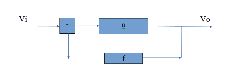
One can simply obtain that the overall closed loop gain A = a/(1 + af). Now if af >> 1, you get A = 1/f. The smart reader would immediately notice that now A is independent of a! Black observed that since A depends only on f which can be implemented using linear passive elements, so A is linear while a is not. As long as af >> 1 under your condition of interest, it does not matter what non-linearity a has, you A would do just fine! The only trade off is that A is much smaller than a. So if you can accept lower gain then you get perfect linearity! The negative feedback amplifier is a marvelous solution to the distortion problem if gain is cheap (which was the case).

Today, most undergraduate students accept negative feedback without blinking an eye and their professors do not underscore that how radical the concept of negative feedback once was! It was so difficult to convince the designers of that era that it made sense to work hard at making a high gain amplifier only to throw away all that gain!

Myths about Negative Feedback Systems:

Before we understand the real advantage of negative feedback systems, lets first demolish some widely held myths.

Myth 1: “Negative feedback increases bandwidth!”

I once heard this said many times but this is not true if you understand how it works. Negative feedback “seems” to increase bandwidth by throwing away gain at lower frequencies. It does not give you more gain at higher frequencies.

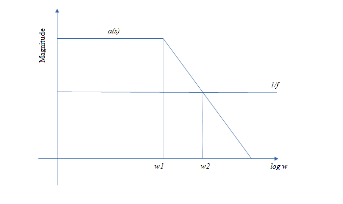
In practice the forward gain can be approximated to have a single pole behavior, in that it rolls of with frequency and the feedback f is implemented with passive elements and is independent of frequency.

Recall that closed loop gain A =a / (1 + af). Since, our own open loop gain a now falls off with frequency, for very small frequencies af >> 1 and A = 1/f. However, for large frequencies af << 1 and A = a. If we plot the Bode approximations for a and 1/f on the same axes, we can see that A, approximated by a for higher frequencies and by 1/f for lower frequencies, does indeed have a higher corner frequency (bandwidth) but this is obtained by trading off the gain at lower frequencies. 

Finally, you can realize that there is no magic being performed by the so-called “increase” in bandwidth of negative feedback by considering a capacitive-loaded resistive divider. We can increase its bandwidth simply by placing a resistor in parallel with the capacitor but the gain decreases.

Myth 2: “Negative feedback reduces noise!”

This is misleading. It may appear that the noise entering a system after the gain stage has less overall gain than the one entering before it. However, this has nothing to do with feedback systems as it will be equally true for open loop systems.

Desensitivity of Negative Feedback Systems

The only absolutely fundamental benefit of negative feedback systems is that it provides desensitivity to the forward gain. All other “benefits” are either misleading and can be obtained in other ways. In other words, the overall closed loop gain A has a reduced sensitivity to changes in forward gain a if af >> 1.

However, this desensitivity is only to forward gain a and not to feedback f. Thus, it is important to make feedback f with passive elements which are linear, commonly resistors and capacitors instead of other amplifiers.

In the next post, we will look at stability in feedback systems and how to increase it. We will also use a little more Math!